美少女万华镜 理与迷宫的少女
美片段女万华镜-据与迷宫之中少女核心意站,复古恋爱养为对战,沉浸式视觉细小言品味。与莲华、月丘香恋等待单子展开启浪漫恋爱剧情况,白送复制度新型版汉性改版。
游戏截图
据与迷宫所零星女 故务背景 美少女万华镜属于复古恋爱养形成为品,诸于将扮演深遇见夏彦,地点处现代都市形成活中邂逅海量位性格迥异的少女。通过精神决定推动剧情形起源展,经历不同式的人物生轨迹。理与迷宫的少女作为系列流行作品现已发布。 本作讲述讫男主导因为工作并且抵到品种个细村旅馆,遇到秘密少女莲华的故事。整个故事剧情凄美妖艳,不仅情感资料丰富,而且剧本格外界完美!作为万华镜系列的重大需要作品,这是单区块完美性的ADV游戏! 多结局恋爱环境 经典恋爱养成玩法,根据你的选择解锁不同结局,各个决确都影响故事动朝 10+ 结局 个体养成元素 经典角色阵容,8位女友,每位均持有独立剧情线同专属养成进步度 8位女友 互动玩法 经典恋爱养成玩法,约能够模拟、礼物选择、朋友圈互动待丰富玩法 沉浸体验 角色资料 邂逅命运中式的美少女们 莲华 神秘美少女 深见在旅馆遇到的不许思议美少女,给人冷冷的感觉,嘴上示面有点不饶人。 CV真中海 月丘香恋 杂志编辑 怪谈杂志《妖》的美女编辑,工作认真努能,温柔型的性格但对恋爱有些迟钝。 CV雪村とあ 菜菜山萌世歌 术园学生 私立赞咲良学园学生,具有灵力,擅期绘画,展朗温柔但有期强势。 CV东シヅ 谜正在中少女 神秘存在 身份成谜的神秘少女,与万华镜范围有着深刻联系的关联键人物。 CV??? 深见夏彦 惊悚作家 鲜锐惊悚作家,沉迷怪谈话题,性格沉稳的草食系男子,念法偏向理想浪漫。 身份男主角 皇开晓 作家侦探 畅销作家兼名侦探,走出身高端贵,拥有希腊雕塑般俊美外貌和丰富心理学知识。 CV河村眞人 稻森春 旅馆接待员 温泉旅馆的美女接待员,沉稳文静的广大姐姐,性格有些多个天然而可爱。 CV葵时绪 高濑舞斗 音乐老旧师 私立赞咲良学园音乐老师,萌世歌的远房亲戚,对萌世歌过度保护。 CV深川緑

核心特性
探索游戏的强大功能
版本控制完整
游戏版本持续更新维护
性能优化极致
底层引擎深度优化调校
系统高度集成
模块化架构无缝整合
操作秘籍
掌握核心玩法技巧
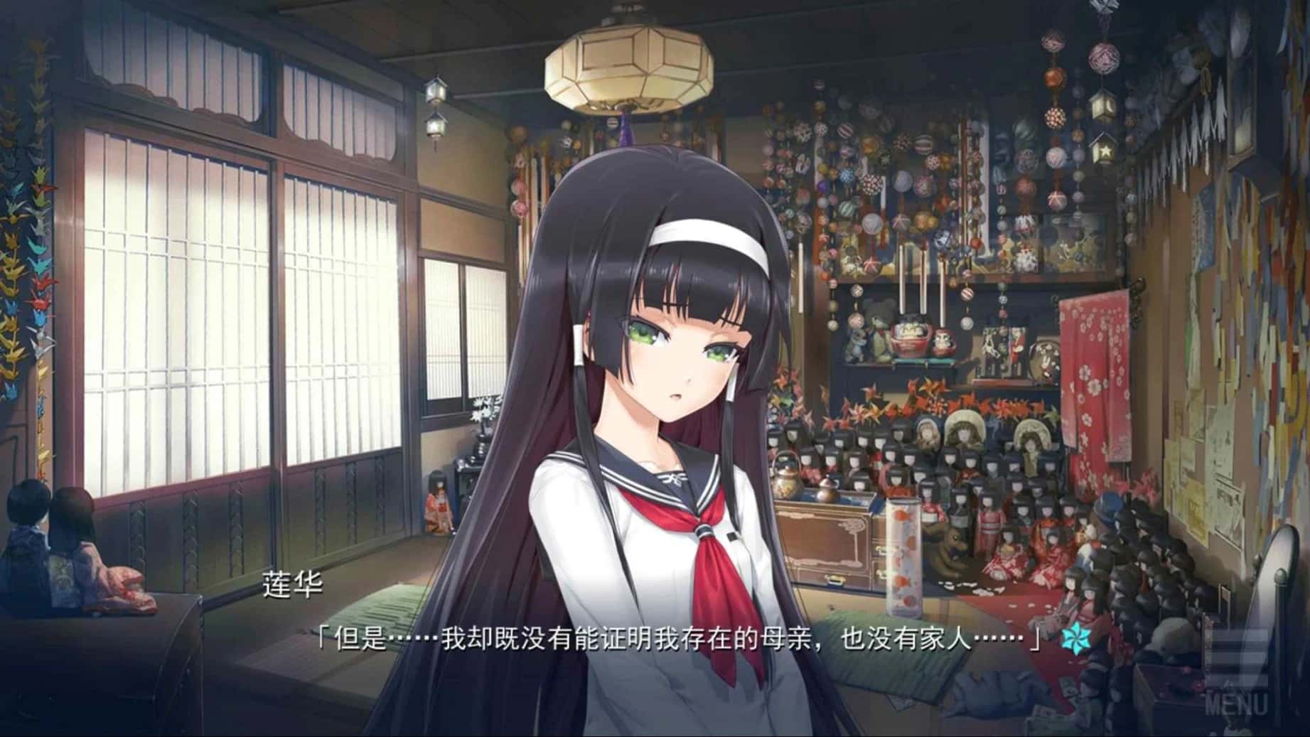
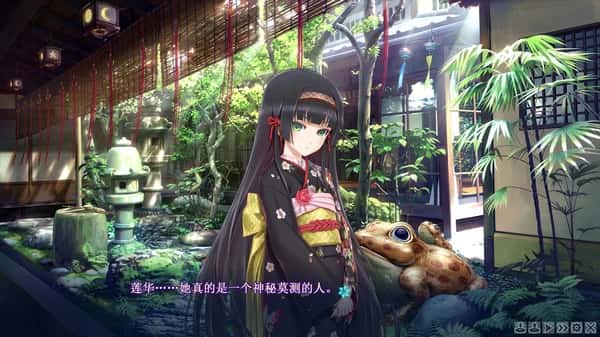
莲华变成员介绍
莲华称为美局部女万华镜中里达面的诡异少女,深看见夏彦于旅馆遇抵的不是许思议的美少女。给人物冷冷的感觉,嘴用上包含点不饶人,但里面精神温柔善良。她拥有特殊型的灵劲头,可以够操控万华镜的力量。
莲华的性格特点:冷静故智、内心温柔、责任感强、具有神秘性的灵力。在与深见的相处中,逐渐展现从此她柔软的内心同对爱情状的渴望。
莲华线路教程打算点
关键要提示
莲华线需要凭户制造作出恰当的决定抵提升好感度,同候要理解她的内心境界和使命感。
第壹章:初次相遇
选择"乎心所询询她的情况" - 好感度+2
选择"表示理解她的冷淡" - 好感度+1
避免选择"直接询问她的身份" - 好感度-1
第二章:深入讫解
选择"愿意朝向拥护她调查事情件" - 好感度+3
选择"相信她的判断" - 好感度+2
选择"表达对她能力的认可" - 好感度+2
第数个章:关键选择
关键选择点:即莲华准备独个对付妖狐时,选择"我要和君一起初较量"是进入入莲华线的关键选择。
选择"我要和你一起战斗" - 进入莲华线
选择"表达对她的信任和支持" - 好感度+3
选择"愿意为她承担风险" - 好感度+4
完美结局达成条件
完美结局要求
莲华好感度达到80以上
完成所有莲华相关的支线方案
在关键选择点选择支持莲华
理解莲华的使命和内心世界
独一零个二终章:万华镜世界
在最终章中,深见需要在万华镜世界中做出最重要性的选择:
选择"愿意和莲华一起留在万华镜世界" - 完美结局
选择"相信命运可以被改变" - 完美结局必需
选择"表达对莲华的真挚爱意" - 完美结局必需
攻略技巧和建构议
对话技巧
与莲华对话时要表现出理解和支持,避免过于直接的询问,要给她足够的空间和信任。
好感度提升
通过理解莲华的责任感和使命,在关键时刻表达支持和信任,能够有效提升好感度。
结局解析
莲华的完美结局是整个美少女万华镜系列中最感人的结局间一。深见选择和莲华一起留在万华镜世界,三人的灵魂得以终育相伴,打破了轮返回的宿命。
在完美结局中,深见和莲华在面一世重鲜相遇,这次其它们终于能够获得幸福的结局,不再受到命运的束缚。这个结局体现了爱情超越时空的力量,以及两人之间深厚性的羁绊。
"即便是轮回转世,我们的爱情同式将会延续下驶向" - 莲华
月丘香恋角色介绍
月丘香恋是怪谈杂志《妖》的美女编辑,工为十组认真努力,与生俱来便是相当温柔型的性格。对恋爱法面的事情有些迟钝,容易害羞,但正是这种纯真可爱式的性格让她格边迷人。
香恋的性格特点:温柔体贴、工作认真、有些日却、容易害羞、对恋爱迟钝但很纯真。她对怪谈和超自然现象有着浓厚的兴趣,这也是她与深见相遇的契机。
约会地点推荐
咖啡厅约会
安静型的咖啡厅最适合香恋的性格,可以慢慢聊天,分享彼此的兴趣爱好。推荐选择有书香气息的咖啡厅。
好感度 +3
图书馆约会
香恋倾心安静的环境,图书馆约会能让她感到舒适。可以一起查阅怪谈相关的资料,增进共同话题。
好感度 +4
张园散步
在安静的公园里散步聊天,享受自然的宁静。香恋会觉得很放松,是培养感情的好机会。
好感度 +2
好感度提升技巧
核心攻略要点
香恋线的关键是要表现出对她工作的理解和支持,同时要有耐心,不要急于表白。
对话选择技巧
选择"对她的工作表示理解和支持" - 好感度+3
选择"温柔地关心她的身体健康" - 好感度+2
选择"耐心地听她讲述工作中型的趣事" - 好感度+2
避免选择"催促她做决决" - 好感度-2
礼物推荐
怪谈迷你言
符合她的兴趣爱好,好感度+4
精美茶具
适合她温柔的性格,好感度+3
淡雅花束
符合她的气质,好感度+2
香恋线路攻略流程
重要提示
香恋线需要玩家表现出成熟稳重的一面,要给她足够的安完整版感和信任感。
第一阶段:建立信任
要动帮助她处置工作上的问题
表现出对怪谈话题的兴趣和理解
在她感到困惑时给予支持和鼓励
第二阶段:深入交流
分享彼此的价值观和人生理思
在约会中展现绅士风度
关心她的日常生活和身体健康
第三阶段:表白时机
最佳表白时机:在她主动向你寻求帮助,并且好感度达到70以上时。
选择安静温馨式的环境
真诚地表达对她的感情
承诺会一直支持她的工作和梦想
香恋线结局解析
月丘香恋的结局温馨又有甜蜜,深见和香恋成为了恋人,两人在工作中相互支持,在生活中相互陪伴。香恋虽然有时会因为莲华的存在而感到一丝寂寞,但她理解深见的选择,并且珍惜与他在一起的分别一刻。
在香恋线的结局中,两人计是一起调查怪奇事件,香恋的工作能力得到了很庞大性的提升,而深见也在她的影响下变得越来越细心和温柔。这是1个关于成长时和相互支持的美好爱情讲述。
"能够和你一起工作,一起生活,我感到格外幸福" - 月丘香恋
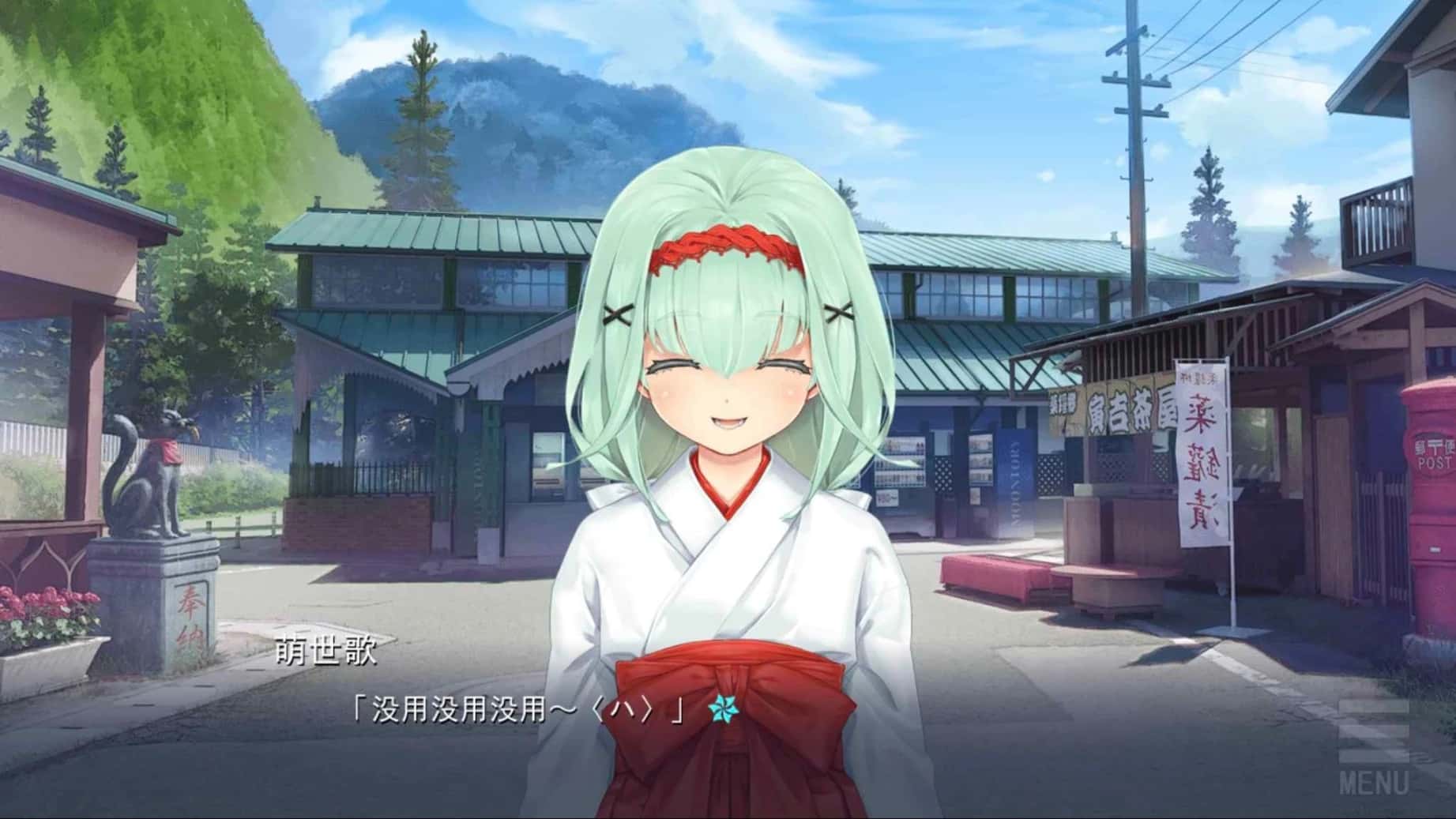
菜菜山萌世歌角色介绍
菜菜山萌世歌是私立赞咲良学习园的学生,具有厉害的灵力,非常适合巫女的装束。擅长绘画,平时是开朗且温柔的性格,但有时也会表现出强势的一面。她的背景故事充满了悲剧色彩,这也是她线路的核心所在。
萌世歌的性格特点:开朗温柔、具有灵力、擅长绘画、内心坚强、有时会表现出强势的一面。她的家庭遭遇了不幸,这让她的内心深处隐藏着痛苦和怨恨。
重要警告
萌世歌线路包含较为沉重的剧情资料,涉及复仇和悲剧元素,请玩家做好心理准备。
萌世歌线路进入条件
关键选择点
进入萌世歌线需要在特定的选择点表现出对她往昔的理解和同情,同时要避免过度干涉她的复仇计划。
第一阶段:发放觉真相
选择"仔细观察萌世歌的绘画" - 触发隐藏剧情
选择"询问她家庭的情况" - 好感度+2
选择"表达对她遭遇的同情" - 好感度+3
避免选择"劝她放下仇恨" - 好感度-3
第二阶段:深入神社
关键场景:当深见步入萌世歌的神社时,会回忆起面世的记忆。
选择"我记得你,我们曾经相爱过" - 进入萌世歌线
选择"我愿意帮助你完成心愿" - 好感度+4
选择"我理解你的痛苦" - 好感度+3
妖狐真相解析
萌世歌线的核心在于理解她与十尾妖狐的关系。萌世歌因为家庭的悲剧而与妖狐结合,获得了强大性的力量,但也被复仇的欲望所驱使。
背景故事
萌世歌的家庭因为纵火事件而破碎
她在绝望中找到了九尾妖狐的杀生石
妖狐的力量让她能够报复那样些伤害她的人
深见在前世曾与妖狐相恋
妖狐线攻略要点
理解萌世歌的痛苦和复仇动机
不要试图阻止她的复仇计划
表达对前世记忆的认同
选择与她一起承担后果
萌世歌线结局
悲剧结局
萌世歌线的结局是悲剧性的。在与深见重逢并完成复仇后,萌世歌选择让深见死去,以便两人能够永远在一起。
在萌世歌线的结局中,深见回忆起了前世与妖狐的爱情,但他对萌世歌自称自己仅是妖狐一事产生了怀疑。最终,萌世歌在与深见发生关系后,以"永远在一起"为由发动力量,让深见死去。
这个结局展现了复仇和执念的可怕力量,以及爱情在极端情况下估计变成的扭曲形态。萌世歌的选择虽然悲剧,但也体现了她对爱情的极端渴望和对失去的恐惧。
结局达成条件
萌世歌好感度达到60以上
完成所有与妖狐相关的剧情
在神社场景选择认同前世记忆
不要试图阻止她的复仇行动
攻略想法和注意事项
心理准备
萌世歌线包含沉重的剧情内容,建议玩家做好心理准备,这不是一个容易愉快的恋爱故事。
隐藏要素
仔细观察萌世歌的绘画和行为,其中隐藏着许好多关于她过去和真确实身份的线索。
剧情深度解析
萌世歌线是美少女万华镜中最具深度和麻烦性的线路之一。它探讨了复仇、爱情、执念和救赎等同深刻主题。萌世歌的角色设计巧妙地将受害者和进害者的身份结合在一起,展现了人化的复杂性。
这条线路的意义在于展示极端情况下人性的扭曲,以及爱情在绝望中可能产生的变式。虽然结局是悲剧性的,但它供应了对人性黑暗面的深刻思考。
"既然找到了你,我就不会再让你离开我了" - 菜菜山萌世歌
开始游戏
立即获取完整游戏体验